Graphs, Kites and Darts – and Theorems

We continue our exploration of properties of Penrose’s aperiodic tilings with kites and darts using Haskell and Haskell Diagrams.

In this blog we discuss some interesting properties we have discovered concerning the , , and operations along with some proofs.

Index

1. Quick Recap (including operations , , on Tgraphs)
2. Composition Problems and a Compose Force Theorem (composition is not a simple inverse to decomposition)
3. Perfect Composition Theorem (establishing relationships between , , )
4. Multiple Compositions (extending the Compose Force theorem for multiple compositions)
5. Proof of the Compose Force Theorem (showing is total on forced Tgraphs)

1. Quick Recap

Haskell diagrams allowed us to render finite patches of tiles easily as discussed in Diagrams for Penrose tiles. Following a suggestion of Stephen Huggett, we found that the description and manipulation of such tilings is greatly enhanced by using planar graphs. In Graphs, Kites and Darts we introduced a specialised planar graph representation for finite tilings of kites and darts which we called Tgraphs (tile graphs). These enabled us to implement operations that use neighbouring tile information and in particular operations , , and .

For ease of reference, we reproduce the half-tiles we are working with here.

Figure 1: Half-tile faces

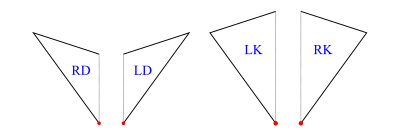
Figure 1 shows the right-dart (RD), left-dart (LD), left-kite (LK) and right-kite (RK) half-tiles. Each has a join edge (shown dotted) and a short edge and a long edge. The origin vertex is shown red in each case. The vertex at the opposite end of the join edge from the origin we call the opp vertex, and the remaining vertex we call the wing vertex.

If the short edges have unit length then the long edges have length (the golden ratio) and all angles are multiples of (a tenth turn) with kite halves having  two 2s and a 1, and dart halves having a 3 and two 1s. This geometry of the tiles is abstracted away from at the graph representation level but used when checking validity of tile additions and by the drawing functions.

There are rules for how the tiles can be put together to make a legal tiling (see e.g. Diagrams for Penrose tiles). We defined a Tgraph (in Graphs, Kites and Darts) as a list of such half-tiles which are constrained to form a legal tiling but must also be connected with no crossing boundaries (see below).

As a simple example consider kingGraph (2 kites and 3 darts round a king vertex). We represent each half-tile as a TileFace with three vertex numbers, then apply makeTgraph to the list of ten Tilefaces. The function makeTgraph :: [TileFace] -> Tgraph performs the necessary checks to ensure the result is a valid Tgraph.

kingGraph :: Tgraph
kingGraph = makeTgraph 
  [LD (1,2,3),RD (1,11,2),LD (1,4,5),RD (1,3,4),LD (1,10,11)
  ,RD (1,9,10),LK (9,1,7),RK (9,7,8),RK (5,7,1),LK (5,6,7)
  ]

To view the Tgraph we simply form a diagram (in this case 2 diagrams horizontally separated by 1 unit)

  hsep 1 [labelled drawj kingGraph, draw kingGraph]

and the result is shown in figure 2 with labels and dashed join edges (left) and without labels and join edges (right).

Figure 2: kingGraph with labels and dashed join edges (left) and without (right).

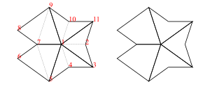
The boundary of the Tgraph consists of the edges of half-tiles which are not shared with another half-tile, so they go round untiled/external regions. The no crossing boundary constraint (equivalently, locally tile-connected) means that a boundary vertex has exactly two incident boundary edges and therefore has a single external angle in the tiling. This ensures we can always locally determine the relative angles of tiles at a vertex. We say a collection of half-tiles is a valid Tgraph if it constitutes a legal tiling but also satisfies the connectedness and no crossing boundaries constraints.

Our key operations on Tgraphs are , , and which are illustrated in figure 3.

Figure 3: decompose, force, and compose

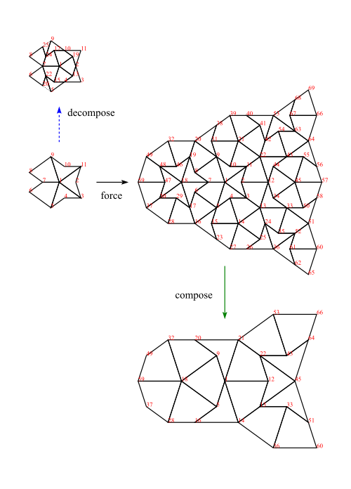
Figure 3 shows the kingGraph with its decomposition above it (left), the result of forcing the kingGraph (right) and the composition of the forced kingGraph (bottom right).

Decompose

An important property of Penrose dart and kite tilings is that it is possible to divide the half-tile faces of a tiling into smaller half-tile faces, to form a new (smaller scale) tiling.

Figure 4: Decomposition of (left) half-tiles

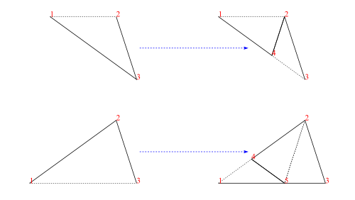
Figure 4 illustrates the decomposition of a left-dart (top row) and a left-kite (bottom row). With our Tgraph representation we simply introduce new vertices for dart and kite long edges and kite join edges and then form the new faces using these. This does not involve any geometry, because that is taken care of by drawing operations.

Force

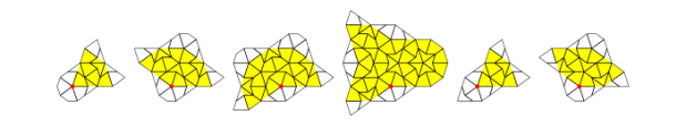
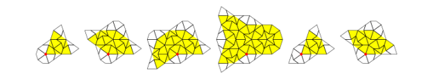
Figure 5 illustrates the rules used by our operation (we omit a mirror-reflected version of each rule).

Figure 5: Force rules

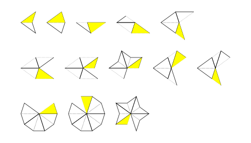
In each case the yellow half-tile is added in the presence of the other half-tiles shown. The yellow half-tile is forced because, by the legal tiling rules and the seven possible vertex types, there is no choice for adding a different half-tile on the edge where the yellow tile is added.

We call a Tgraph correct if it represents a tiling which can be continued infinitely to cover the whole plane without getting stuck, and incorrect otherwise. Forcing involves adding half-tiles by the illustrated rules round the boundary until either no more rules apply (in which case the result is a forced Tgraph) or a stuck tiling is encountered (in which case an incorrect Tgraph error is raised). Hence is a partial function but total on correct Tgraphs.

Compose: This is discussed in the next section.

2. Composition Problems and a Theorem

Compose Choices

For an infinite tiling, composition is a simple inverse to decomposition. However, for a finite tiling with boundary, composition is not so straight forward. Firstly, we may need to leave half-tiles out of a composition because the necessary parts of a composed half-tile are missing. For example, a half-dart with a boundary short edge or a whole kite with both short edges on the boundary must necessarily be excluded from a composition. Secondly, on the boundary, there can sometimes be a problem of choosing whether a half-dart should compose to become a half-dart or a half-kite. This choice in composing only arises when there is a half-dart with its wing on the boundary but insufficient local information to determine whether it should be part of a larger half-dart or a larger half-kite.

In the literature (see for example 1 and 2) there is an often repeated method for composing (also called inflating). This method always make the kite choice when there is a choice. Whilst this is a sound method for an unbounded tiling (where there will be no choice), we show that this is an unsound method for finite tilings as follows.

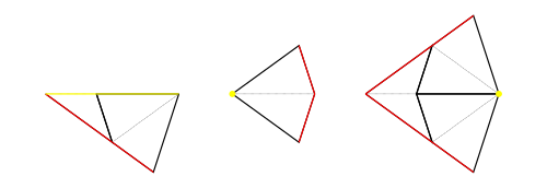
Clearly composing should preserve correctness. However, figure 6 (left) shows a correct Tgraph which is a forced queen, but the kite-favouring composition of the forced queen produces the incorrect Tgraph shown in figure 6 (centre). Applying our function to this reveals a stuck tiling and reports an incorrect Tgraph.

Figure 6: An erroneous and a safe composition

Our algorithm (discussed in Graphs, Kites and Darts) detects dart wings on the boundary where there is a choice and classifies them as unknowns. Our composition refrains from making a choice by not composing a half dart with an unknown wing vertex. The rightmost Tgraph in figure 6 shows the result of our composition of the forced queen with the half-tile faces left out of the composition (the remainder faces) shown in green. This avoidance of making a choice (when there is a choice) guarantees our composition preserves correctness.

Compose is a Partial Function

A different composition problem can arise when we consider Tgraphs that are not decompositions of Tgraphs. In general, is a partial function on Tgraphs.

Figure 7: Composition may fail to produce a Tgraph

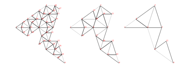
Figure 7 shows a Tgraph (left) with its sucessful composition (centre) and the half-tile faces that would result from a second composition (right) which do not form a valid Tgraph because of a crossing boundary (at vertex 6). Thus composition of a Tgraph may fail to produce a Tgraph when the resulting faces are disconnected or have a crossing boundary.

However, we claim that is a total function on forced Tgraphs.

Compose Force Theorem

Theorem: Composition of a forced Tgraph produces a valid Tgraph.

We postpone the proof (outline) for this theorem to section 5. Meanwhile we use the result to establish relationships between , , and in the next section.

3. Perfect Composition Theorem

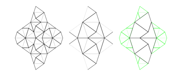
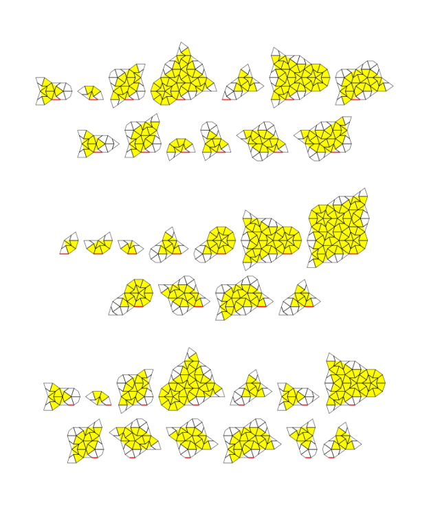
In Graphs, Kites and Darts we produced a diagram showing relationships between multiple decompositions of a dart and the forced versions of these Tgraphs. We reproduce this here along with a similar diagram for multiple decompositions of a kite.

Figure 8: Commuting Diagrams

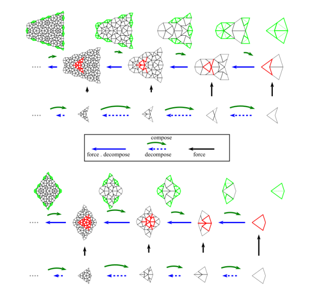
In figure 8 we show separate (apparently) commuting diagrams for the dart and for the kite. The bottom rows show the decompositions, the middle rows show the result of forcing the decompositions, and the top rows illustrate how the compositions of the forced Tgraphs work by showing both the composed faces (black edges) and the remainder faces (green edges) which are removed in the composition. The diagrams are examples of some commutativity relationships concerning , and which we will prove.

It should be noted that these diagrams break down if we consider only half-tiles as the starting points (bottom right of each diagram). The decomposition of a half-tile does not recompose to its original, but produces an empty composition. So we do not even have in these cases. Forcing the decomposition also results in an empty composition. Clearly there is something special about the depicted cases and it is not merely that they are wholetile complete because the decompositions are not wholetile complete. [Wholetile complete means there are no join edges on the boundary, so every half-tile has its other half.]

Below we have captured the properties that are sufficient for the diagrams to commute as in figure 8. In the proofs we use a partial ordering on Tgraphs (modulo vertex relabelling) which we define next.

Partial ordering of Tgraphs

If and are both valid Tgraphs and consists of a subset of the (half-tile) faces of we have

which gives us a partial order on Tgraphs. Often, though, is only isomorphic to a subset of the faces of , requiring a vertex relabelling to become a subset. In that case we write

which is also a partial ordering and induces an equivalence of Tgraphs defined by

in which case and are isomorphic as Tgraphs.

Both and are monotonic with respect to meaning:

We also have is monotonic, but only when restricted to correct Tgraphs. Also, when restricted to correct Tgraphs, we have is non decreasing because it only adds faces:

and is idempotent (forcing a forced correct Tgraph leaves it the same):

Composing perfectly and perfect compositions

Definition: A Tgraph composes perfectly if all faces of are composable (i.e there are no remainder faces of when composing).

We note that the composed faces must be a valid Tgraph (connected with no crossing boundaries) if all faces are included in the composition because has those properties. Clearly, if composes perfectly then

In general, for arbitrary where the composition is defined, we only have

Definition: A Tgraph is a perfect composition if composes perfectly.

Clearly if is a perfect composition then

(We could use equality here because any new vertex labels introduced by will be removed by ). In general, for arbitrary ,

Lemma 1: is a perfect composition if and only if has the following 2 properties:

1. every half-kite with a boundary join has either a half-dart or a whole kite on the short edge, and
2. every half-dart with a boundary join has a half-kite on the short edge,

(Proof outline:) Firstly note that unknowns in (= ) can only come from boundary joins in . The properties 1 and 2 guarantee that has no unknowns. Since every face of has come from a decomposed face in , there can be no faces in that will not recompose, so will compose perfectly to . Conversely, if is a perfect composition, its decomposition can have no unknowns. This implies boundary joins in must satisfy properties 1 and 2.

(Note: a perfect composition may have unknowns even though its decomposition has none.)

It is easy to see two special cases:

1. If is wholetile complete then is a perfect composition.Proof: Wholetile complete implies no boundary joins which implies properties 1 and 2 in lemma 1 which implies is a perfect composition.
2. If is a decomposition then is a perfect composition.Proof: If is a decomposition, then every half-dart has a half-kite on the short edge which implies property 2 of lemma 1. Also, any half-kite with a boundary join in must have come from a decomposed half-dart since a decomposed half-kite produces a whole kite with no boundary kite join. So the half-kite must have a half-dart on the short edge which implies property 1 of lemma 1. The two properties imply is a perfect composition.

We note that these two special cases cover all the Tgraphs in the bottom rows of the diagrams in figure 8. So the Tgraphs in each bottom row are perfect compositions, and furthermore, they all compose perfectly except for the rightmost Tgraphs which have empty compositions.

In the following results we make the assumption that a Tgraph is correct, which guarantees that when is applied, it terminates with a correct Tgraph. We also note that preserves correctness as does (provided the composition is defined).

Lemma 2: If is a forced, correct Tgraph then

(Proof outline:) The proof uses a case analysis of boundary and internal vertices of . For internal vertices we just check there is no change at the vertex after using figure 11 (plus an extra case for the forced star). For boundary vertices we check local contexts similar to those depicted in figure 10 (but including empty composition cases). This reveals there is no local change of the boundary at any boundary vertex, and since this is true for all boundary vertices, there can be no global change. (We omit the full details).

Lemma 3: If is a perfect composition and a correct Tgraph, then

(Proof outline:) The proof is by analysis of each possible force rule applicable on a boundary edge of and checking local contexts to establish that (i) the result of applying to the local context must include the added half-tile, and (ii) if the added half tile has a new boundary join, then the result must include both halves of the new half-tile. The two properties of perfect compositions mentioned in lemma 1 are critical for the proof. However, since the result of adding a single half-tile may break the condition of the Tgraph being a pefect composition, we need to arrange that half-tiles are completed first then each subsequent half-tile addition is paired with its wholetile completion. This ensures the perfect composition condition holds at each step for a proof by induction. [A separate proof is needed to show that the ordering of applying force rules makes no difference to a final correct Tgraph (apart from vertex relabelling)].

Lemma 4 If composes perfectly and is a correct Tgraph then

Proof: Assume composes perfectly and is a correct Tgraph. Since is non-decreasing (with respect to on correct Tgraphs)

and since is monotonic

Since composes perfectly, the left hand side is just , so

and since is monotonic (with respect to on correct Tgraphs)

For the opposite direction, we substitute for in lemma 3 to get

Then, since , we have

Apply to both sides (using monotonicity)

For any for which the composition is defined we have so we get

Now apply to both sides and note to get

Combining this with (*) above proves the required equivalence.

Theorem (Perfect Composition): If composes perfectly and is a correct Tgraph then

Proof: Assume composes perfectly and is a correct Tgraph. By lemma 4 we have

Applying to both sides, gives

Now by lemma 2, with 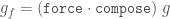, the right hand side is equivalent to

which establishes the result.

Corollaries (of the perfect composition theorem):

1. If is a perfect composition and a correct Tgraph then
   

   Proof: Let (so ) in the theorem.

   [This result generalises lemma 2 because any correct forced Tgraph is necessarily wholetile complete and therefore a perfect composition, and .]

2. If is a perfect composition and a correct Tgraph then
   

   Proof: Apply to both sides of the previous corollary and note that

   

   provided the composition is defined, which it must be for a forced Tgraph by the Compose Force theorem.

3. If is a perfect composition and a correct Tgraph then
   

   Proof: Apply to both sides of the previous corollary noting is monotonic and idempotent for correct Tgraphs

   

   From the fact that is non decreasing and and are monotonic, we also have

   

   Hence combining these two sub-Tgraph results we have

   

   

It is important to point out that if is a correct Tgraph and is a perfect composition then this is not the same as composes perfectly. It could be the case that has more faces than and so could have unknowns. In this case we can only prove that

As an example where this is not an equivalence, choose to be a star. Then its composition is the empty Tgraph (which is still a pefect composition) and so the left hand side is the empty Tgraph, but the right hand side is a sun.

Perfectly composing generators

The perfect composition theorem and lemmas and the three corollaries justify all the commuting implied by the diagrams in figure 8. However, one might ask more general questions like: Under what circumstances do we have (for a correct forced Tgraph )

Definition A generator of a correct forced Tgraph is any Tgraph such that and .

We can now state that

Corollary If a correct forced Tgraph has a generator which composes perfectly, then

Proof: This follows directly from lemma 4 and the perfect composition theorem.

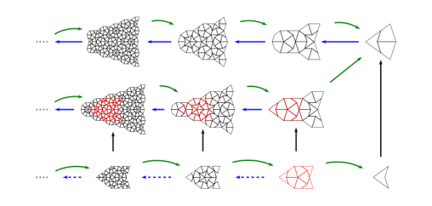
As an example where the required generator does not exist, consider the rightmost Tgraph of the middle row in figure 9. It is generated by the Tgraph directly below it, but it has no generator with a perfect composition. The Tgraph directly above it in the top row is the result of applying which has lost the leftmost dart of the Tgraph.

Figure 9: A Tgraph without a perfectly composing generator

We could summarise this section by saying that can lose information which cannot be recovered by a subsequent and, similarly, can lose information which cannot be recovered by a subsequent . We have defined perfect compositions which are the Tgraphs that do not lose information when decomposed and Tgraphs which compose perfectly which are those that do not lose information when composed. Forcing does the same thing at each level of composition (that is it commutes with composition) provided information is not lost when composing.

4. Multiple Compositions

We know from the Compose Force theorem that the composition of a Tgraph that is forced is always a valid Tgraph. In this section we use this and the results from the last section to show that composing a forced, correct Tgraph produces a forced Tgraph.

First we note that:

Lemma 5: The composition of a forced, correct Tgraph is wholetile complete.

Proof: Let where is a forced, correct Tgraph. A boundary join in implies there must be a boundary dart wing of the composable faces of . (See for example figure 4 where this would be vertex 2 for the half dart case, and vertex 5 for the half-kite face). This dart wing cannot be an unknown as the half-dart is in the composable faces. However, a known dart wing must be either a large kite centre or a large dart base and therefore internal in the composable faces of (because of the force rules) and therefore not on the boundary in . This is a contradiction showing that can have no boundary joins and is therefore wholetile complete.

Theorem: The composition of a forced, correct Tgraph is a forced Tgraph.

Proof: Let for some forced, correct Tgraph , then is wholetile complete (by lemma 5) and therefore a perfect composition. Let , so composes perfectly (). By the perfect composition theorem we have

We also have

Applying to both sides, noting that is monotonic and the identity on forced Tgraphs, we have

Applying to both sides, noting that is monotonic, we have

By (**) above, the left hand side is equivalent to so we have

but since we also have ( being non-decreasing)

we have established that

which means is a forced Tgraph.

This result means that after forcing once we can repeatedly compose creating valid Tgraphs until we reach the empty Tgraph.

We can also use lemma 5 to establish the converse to a previous corollary:

Corollary If a correct forced Tgraph satisfies:

then has a generator which composes perfectly.

Proof: By lemma 5, is wholetile complete and hence a perfect composition. This means that composes perfectly and it is also a generator for because

5. Proof of the Compose Force theorem

Theorem (Compose Force): Composition of a forced Tgraph produces a valid Tgraph.

Proof: For any forced Tgraph we can construct the composed faces. For the result to be a valid Tgraph we need to show no crossing boundaries and connectedness for the composed faces. These are proved separately by case analysis below.

Proof of no crossing boundaries

Assume is a forced Tgraph and that it has a non-empty set of composed faces (we can ignore cases where the composition is empty as the empty Tgraph is valid). Consider a vertex v in the composed faces of and first take the case that v is on the boundary of . We consider the possible local contexts for a vertex v on a forced Tgraph boundary and the nature of the composed faces at v in each case.

Figure 10: Forced Boundary Vertex Contexts

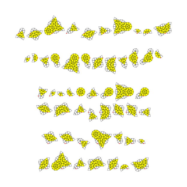
Figure 10 shows local contexts for a boundary vertex v in a forced Tgraph where the composition is non-empty. In each case v is shown as a red dot, and the composition is shown filled yellow. The cases for v are shown in rows: the first row is for dart origins, the second row is for kite origins, the next two rows are for kite wings, and the last two rows are for kite opps. The dart wing cases are a subset of the kite opp cases, so not repeated, and dart opp vertices are excluded because they cannot be on the boundary of a forced Tgraph. We only show left-hand versions, so there is a mirror symmetric set for right-hand versions.

It is easy to see that there are no crossing boundaries of the composed faces at v in each case. Since any boundary vertex of any forced Tgraph (with a non-empty composition) must match one of these local context cases around the vertex, we can conclude that a boundary vertex of cannot become a crossing boundary in .

Next take the case where v is an internal vertex of .

Figure 11: Vertex types and their relationships

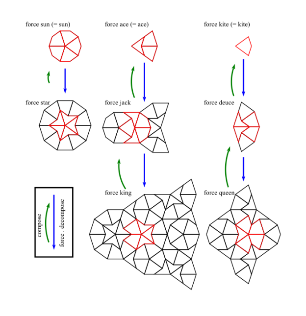
Figure 11 shows relationships between the forced Tgraphs of the 7 (internal) vertex types (plus a kite at the top right). The red faces are those around the vertex type and the black faces are those produced by forcing (if any). Each forced Tgraph has its composition directly above with empty compositions for the top row. We note that a (forced) star, jack, king, and queen vertex remains an internal vertex in the respective composition so cannot become a crossing boundary vertex. A deuce vertex becomes the centre of a larger kite and is no longer present in the composition (top right). That leaves cases for the sun vertex and ace vertex (=fool vertex). The sun Tgraph (sunGraph) and fool Tgraph (fool) consist of just the red faces at the respective vertex (shown top left and top centre). These both have empty compositions when there is no surrounding context. We thus need to check possible forced local contexts for sunGraph and fool.

The fool case is simple and similar to a duece vertex in that it is never part of a composition. [To see this consider inverting the decomposition arrows shown in figure 4. In both cases we see the half-dart opp vertex (labelled 4 in figure 4) is removed].

For the sunGraph there are only 7 local forced context cases to consider where the sun vertex is on the boundary of the composition.

Figure 12: Forced Contexts for a sun vertex v where v is on the composition boundary

Six of these are shown in figure 12 (the missing one is just a mirror reflection of the fourth case). Again, the relevant vertex v is shown as a red dot and the composed faces are shown filled yellow, so it is easy to check that there is no crossing boundary of the composed faces at v in each case. Every forced Tgraph containing an internal sun vertex where the vertex is on the boundary of the composition must match one of the 7 cases locally round the vertex.

Thus no vertex from can become a crossing boundary vertex in the composed faces and since the vertices of the composed faces are a subset of those of , we can have no crossing boundary vertex in the composed faces.

Proof of Connectedness

Assume is a forced Tgraph as before. We refer to the half-tile faces of that get included in the composed faces as the composable faces and the rest as the remainder faces. We want to prove that the composable faces are connected as this will imply the composed faces are connected.

As before we can ignore cases where the set of composable faces is empty, and assume this is not the case. We study the nature of the remainder faces of . Firstly, we note:

Lemma (remainder faces)

The remainder faces of are made up entirely of groups of half-tiles which are either:

1. Half-fools (= a half dart and both halves of the kite attached to its short edge) where the other half-fool is entirely composable faces, or
2. Both halves of a kite with both short edges on the () boundary (so they are not part of a half-fool) where only the origin is in common with composable faces, or
3. Whole fools with just the shared kite origin in common with composable faces.

Figure 13: Remainder face groups (cases 1,2, and 3)

These 3 cases of remainder face groups are shown in figure 13. In each case the border in common with composable faces is shown yellow and the red edges are necessarily on the boundary of (the black boundary could be on the boundary of or shared with another reamainder face group). [A mirror symmetric version for the first group is not shown.] Examples can be seen in e.g. figure 12 where the first Tgraph has four examples of case 1, and two of case 2, the second has six examples of case 1 and two of case 2, and the fifth Tgraph has an example of case 3 as well as four of case 1. [We omit the detailed proof of this lemma which reasons about what gets excluded in a composition after forcing. However, all the local context cases are included in figure 14 (left-hand versions), where we only show those contexts where there is a non-empty composition.]

We note from the (remainder faces) lemma that the common boundary of the group of remainder faces with the composable faces (shown yellow in figure 13) is just a single vertex in cases 2 and 3. In case 1, the common boundary is just a single edge of the composed faces which is made up of 2 adjacent edges of the composable faces that constitute the join of two half-fools.

This means each (remainder face) group shares boundary with exactly one connected component of the composable faces.

Next we establish that if two (remainder face) groups are connected they must share boundary with the same connected component of the composable faces. We need to consider how each (remainder face) group can be connected with a neighbouring such group. It is enough to consider forced contexts of boundary dart long edges (for cases 1 and 3) and boundary kite short edges (for case 2). The cases where the composition is non-empty all appear in figure 14 (left-hand versions) along with boundary kite long edges (middle two rows) which are not relevant here.

Figure 14: Forced contexts for boundary edges

We note that, whenever one group of the remainder faces (half-fool, whole-kite, whole-fool) is connected to a neighbouring group of the remainder faces, the common boundary (shared edges and vertices) with the compososable faces is also connected, forming either 2 adjacent composed face boundary edges (= 4 adjacent edges of the composable faces), or a composed face boundary edge and one of its end vertices, or a single composed face boundary vertex.

It follows that any connected collection of the remainder face groups shares boundary with a unique connected component of the composable faces. Since the collection of composable and remainder faces together is connected ( is connected) the removal of the remainder faces cannot disconnect the composable faces. For this to happen, at least one connected collection of remainder face groups would have to be connected to more than one connected component of composable faces.

This establishes connectedness of any composition of a forced Tgraph, and this completes the proof of the Compose Force theorem.

References

[1] Martin Gardner (1977) MATHEMATICAL GAMES. Scientific American, 236(1), (pages 110 to 121). http://www.jstor.org/stable/24953856

[2] Grünbaum B., Shephard G.C. (1987) Tilings and Patterns. W. H. Freeman and Company, New York. ISBN 0-7167-1193-1 (Hardback) (pages 540 to 542).